Lesson Objective
By the end of this lesson, you should be able to:
- Define Tree Structures - Explain trees as connected, undirected graphs with no cycles
- Understand Binary Trees - Describe rooted trees where each node has at most two children
- Recognize Tree Applications - Identify real-world uses for rooted trees in computing
- Trace Traversal Algorithms - Follow pre-order, in-order, and post-order traversals
- Apply Tree Concepts - Understand binary search trees and node deletion scenarios
Student Login
Access exclusive lesson resources, notes, and materials.
Introduction to Tree Data Structures
A tree is a fundamental hierarchical data structure used across many computing areas. Formally, it is a connected, undirected graph with no cycles, meaning there is exactly one unique path between any two nodes.
Key Tree Concepts
Rooted Trees: Most practical trees are rooted, with one node designated as the root from which all other nodes descend.
- Root: The topmost node (no parent)
- Parent: A node that has child nodes
- Child: A node directly connected below a parent
- Leaf: A node with no children
- Subtree: A tree consisting of a node and its descendants
- Depth: Distance from root to a node
- Height: Maximum depth of any node in the tree
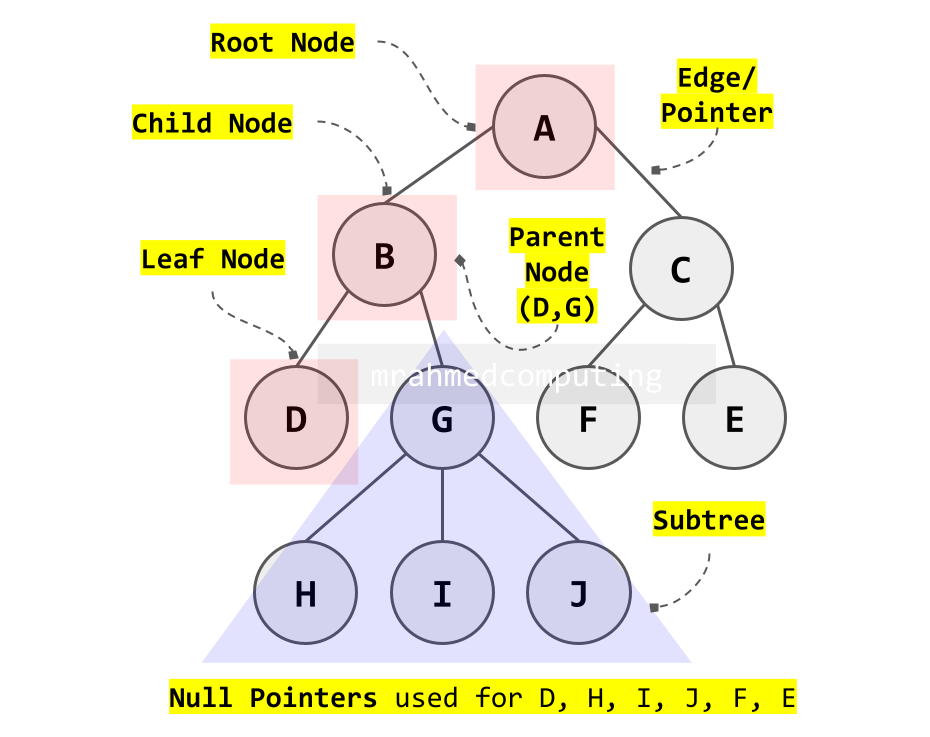
Important Property: Every node except the root has exactly one unique parent node.
Binary Trees
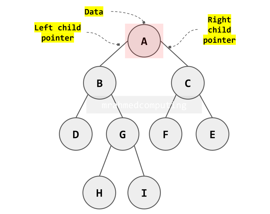
Binary Node Structure
Each node in a binary tree consists of three parts:
- Data: The value stored (can be primitive or complex)
- Left Pointer: Reference to the left child node
- Right Pointer: Reference to the right child node
A binary tree is a specialized rooted tree where each node has at most two children, conventionally called the left child and right child.
Binary Tree Memory Representation
This dictionary represents a binary tree where keys are node values and values are lists containing left and right children (empty list for leaf nodes).
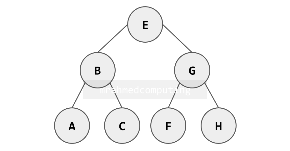
Dictionary Representation (Python Example):
BinaryTree = {
    "E": ["B", "G"],
    "B": ["A", "C"],
    "G": ["F", "H"],
    "A": [],
    "C": [],
    "F": [],
    "H": []
}
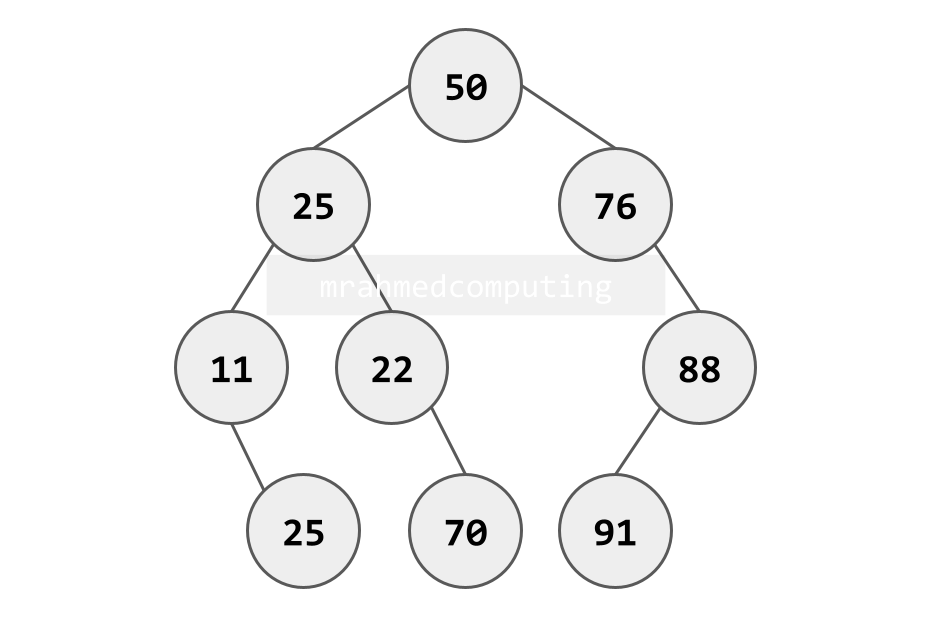
Binary Tree Implementation Methods
Here is another Binary Tree. This binary tree will be used in the following linked list and array examples. The root node of this tree contains the data value 50. There are a number of parent and child nodes.
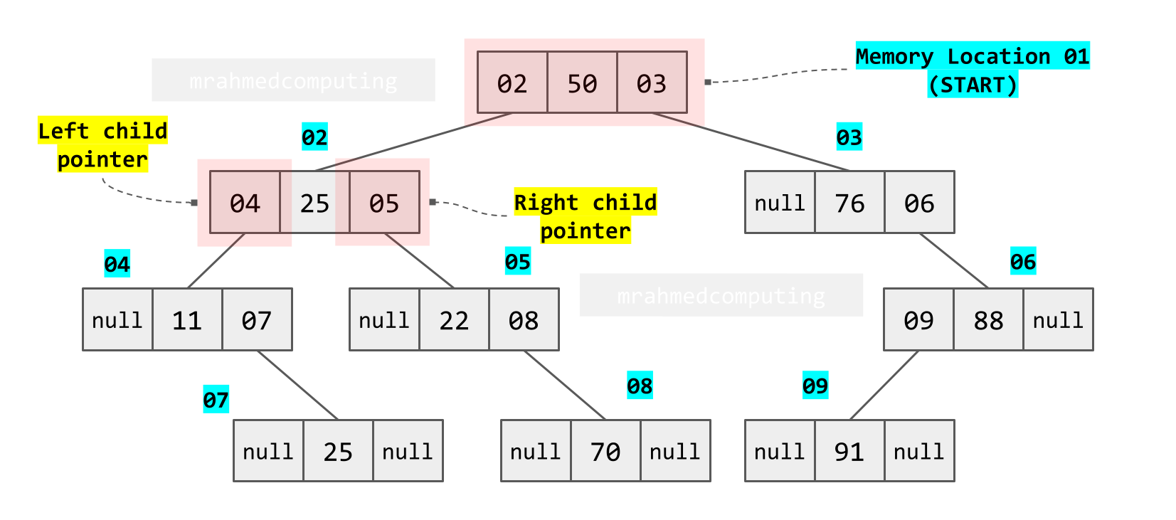
Linked List Implementation:
- Nodes stored dynamically in memory
- Each node contains data, left pointer, right pointer
- Pointers store memory addresses of child nodes
- Flexible for dynamic tree growth
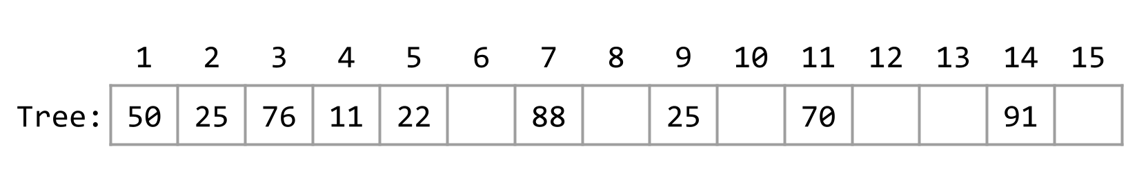
Array Implementation:
- Uses formulas to calculate child positions
- Left Child: position = 2 × parent position
- Right Child: position = 2 × parent position + 1
- Parent/Root: position = child position // 2 (integer division)
- Efficient for complete binary trees, wastes space for sparse trees
| Parent Position | Left Child (2×P) | Right Child (2×P+1) |
|---|---|---|
| 01 | 02 | 03 |
| 02 | 04 | 05 |
| 03 | 06 | 07 |
| X | 2×X | 2×X+1 |
Binary Search Trees (BST)
A binary search tree is a specialized binary tree that maintains a specific ordering property for efficient searching.
When building a binary search tree, nodes are added in the order given, with the first item at the root. Starting at the root each time, if the next item is less than the root, it is added to the left of the root, otherwise, to the right. Apply the same rule at the root of each sub-tree.
BST Properties and Rules
Binary Search Tree Rules:
- Must be a binary tree
- No duplicate values allowed
- For any node:
- All values in the left subtree are less than the node's value
- All values in the right subtree are greater than the node's value
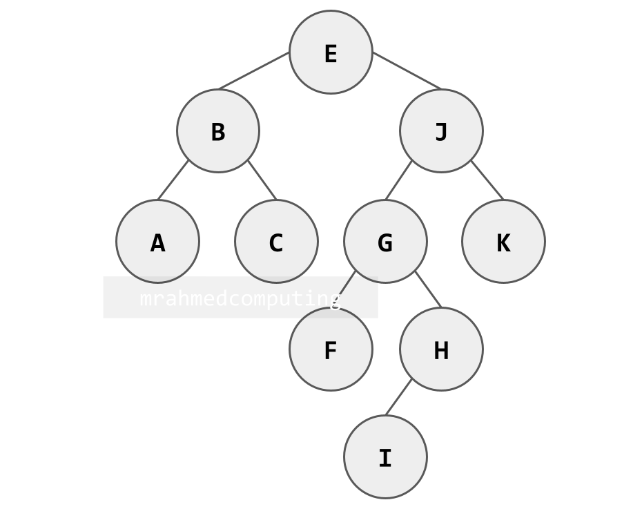
Building a BST (Example: [E, B, J, A, G, H, C, I, F, K]):
- First element 'E' becomes the root
- 'B' < 'E' → goes to left of E
- 'J' > 'E' → goes to right of E
- 'A' < 'E' → goes left, 'A' < 'B' → goes left of B
- Continue applying the same rule at each subtree root
Searching in a BST (Example: Searching for 'H'):
- Start at root 'E': H > E → go right
- At node 'J': H < J → go left
- At node 'G': H > G → go right
- Found at node 'H': H = H → search successful
Note: Image on the right/bottom is animated and shows the different stages of the search.

Binary Tree Traversal Algorithms
Traversal refers to systematically visiting all nodes in a tree. Binary trees support three primary depth-first traversal methods, each producing a different node order.
Traversal Methods and Rules
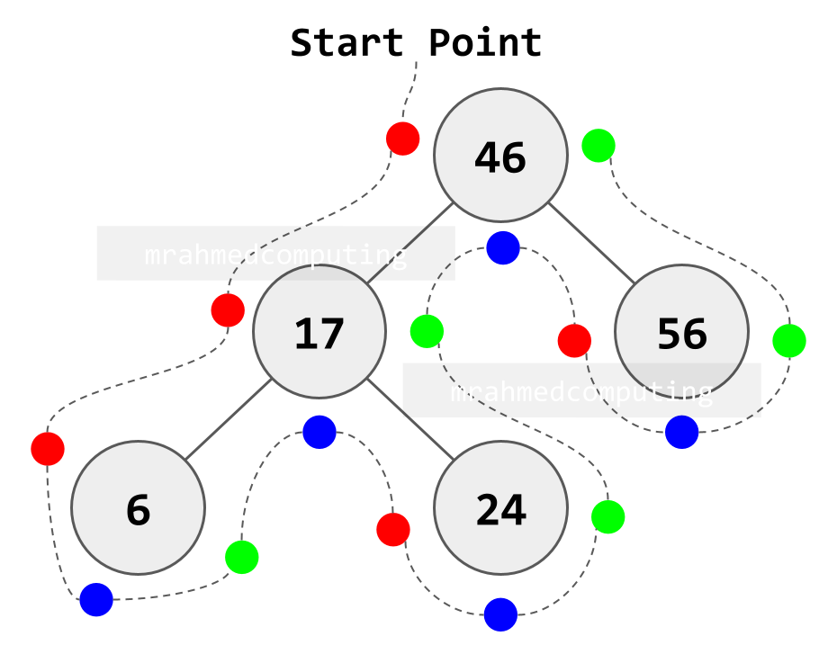
Visualization Technique: Imagine walking around the tree, always keeping it to your left:
- Pre-order: Process node when passing its LEFT side
- In-order: Process node when passing its BOTTOM side
- Post-order: Process node when passing its RIGHT side
1. Pre-order Traversal (Root → Left → Right)
Algorithm:
- Process the root node (R)
- Traverse the left subtree in pre-order
- Traverse the right subtree in pre-order
Note: Image below is animated and shows the different stages of the search.

2. In-order Traversal (Left → Root → Right)
Algorithm:
- Traverse the left subtree in in-order
- Process the root node (R)
- Traverse the right subtree in in-order
Note: Image below is animated and shows the different stages of the search.
Uses: Getting sorted values from a BST, infix expression evaluation.
3. Post-order Traversal (Left → Right → Root)
Algorithm:
- Traverse the left subtree in post-order
- Traverse the right subtree in post-order
- Process the root node (R)
Note: Image below is animated and shows the different stages of the search.

Binary Tree Traversal - Summary
This diagram shows which node to examine in order depending on the traversal being used. You start from the top left of the root node. If you are using Pre-order traversal, you examine the node when you pass from the left. If you are using In-order traversal, you examine the node when you pass the bottom of the node. If you are using Post-order traversal, you examine the node when you pass the right side of the node.
- Pre-order - Left of Node
- In-order - Bottom of Node
- Post-order - Right of Node
Deleting Nodes from a Binary Search Tree
Removing a node from a BST must preserve the binary search tree properties. The approach differs based on how many children the target node has.
Three Deletion Cases
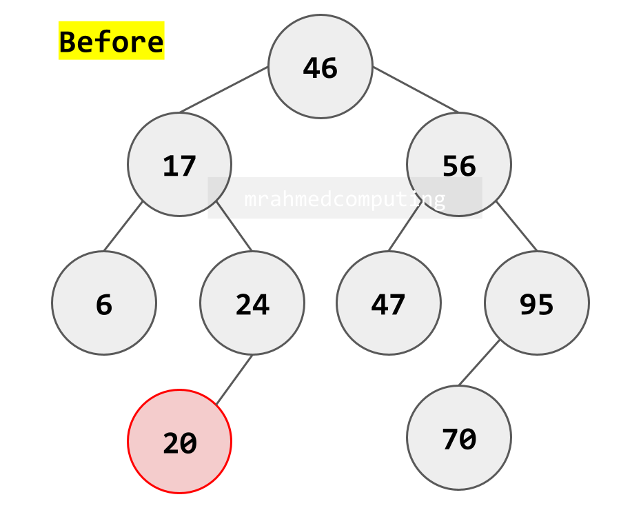
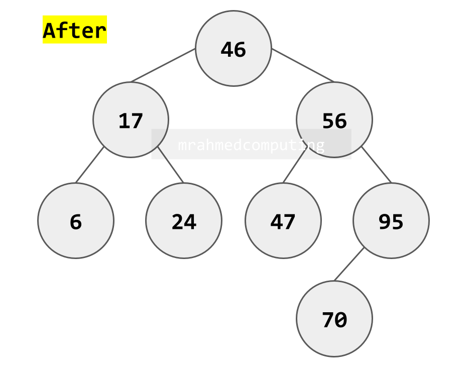
Case 1: Deleting a Leaf Node (No Children)
- Simplest case
- Simply remove the node
- Set the parent's corresponding child pointer to null/None
- BST properties remain intact
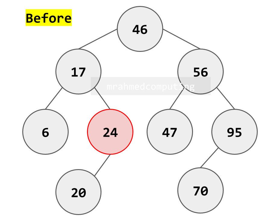
Case 2: Deleting a Node with One Child
- Node has either left OR right child (but not both)
- Remove the node
- Connect the node's parent directly to the node's only child
- "Bypass" the deleted node

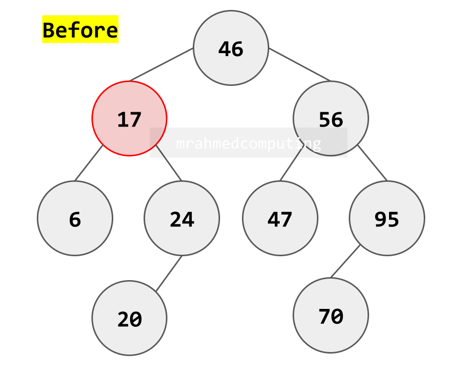
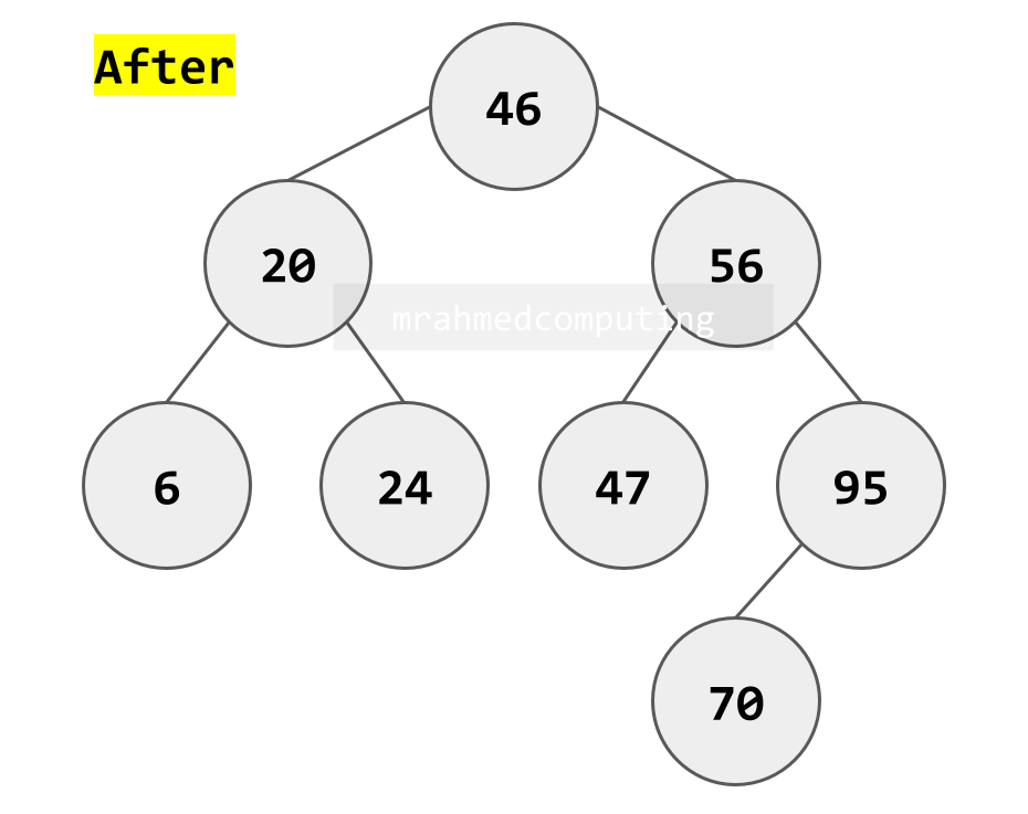
Case 3: Deleting a Node with Two Children
- Most complex case
- Find a replacement node that preserves BST properties
- Two common approaches:
- In-order predecessor: Largest value in left subtree
- In-order successor: Smallest value in right subtree
- Replace the deleted node's value with the replacement's value
- Delete the replacement node (which will be Case 1 or 2)
Real-World Applications of Trees
Tree Applications
Tree data structures are used in a wide variety of applications, including:
- File systems: Tree data structures are used to represent the hierarchical structure of files and directories in file systems. The directory structure on your computer is a tree data structure, with files and subdirectories represented as nodes in the tree.
- Databases: Tree data structures are used to index data in databases, which can improve the efficiency of search and retrieval operations.
- Routers: Tree data structures are used to store routing information in routers, which allows them to efficiently route packets to their destinations. Wireless and wired networks.
- Decision making: Tree data structures can be used to represent decision trees, which are used in artificial intelligence and machine learning to make decisions.
- Sorting and searching: Tree data structures can be used to implement efficient sorting and searching algorithms.
- Compression algorithms: Huffman Coding?
Here are some specific examples of how tree data structures are used in real-world applications:
- The search bar on a website: When you use the search bar on a website, the website's server uses a tree data structure to index the website's content. This allows the server to quickly find the pages that are most relevant to your search query.
- The autocomplete feature on a smartphone: The autocomplete feature on your smartphone uses a tree data structure to store a dictionary of words. This allows the phone to suggest words as you type, which can help you to type more quickly and accurately.
- The spam filter in your email inbox: Your email inbox's spam filter uses a tree data structure to classify emails as spam or not spam. This helps to keep your inbox free of unwanted emails.
- The recommendation engine on a streaming service: The recommendation engine on a streaming service uses a tree data structure to store information about your viewing habits. This allows the service to recommend new shows and movies that you are likely to enjoy.
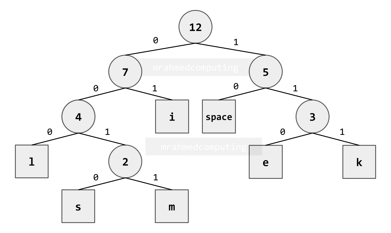
Huffman Coding Example
- Text to Compress: "i like limes" (12 characters)
- Original Size (7-bit ASCII): 12 × 7 = 84 bits
- Compression Process: Build a Huffman tree based on character frequency, assign shorter codes to more frequent characters.
| Character | Frequency | Huffman Code | Bits Used |
|---|---|---|---|
| i | 3 | 2 bits | 3 × 2 = 6 bits |
| space | 2 | 2 bits | 2 × 2 = 4 bits |
| l | 2 | 3 bits | 2 × 3 = 6 bits |
| k | 1 | 3 bits | 1 × 3 = 3 bits |
| e | 2 | 3 bits | 2 × 3 = 6 bits |
| m | 1 | 4 bits | 1 × 4 = 4 bits |
| s | 1 | 4 bits | 1 × 4 = 4 bits |
| Total | 12 | 33 bits |
Compression Result: 84 bits → 33 bits (51 bits saved, 61% reduction)
Lesson Summary
- Tree Definition: Connected, undirected graph with no cycles; unique path between any two nodes
- Binary Tree: Rooted tree where each node has at most two children (left and right)
- Binary Search Tree (BST): Binary tree with ordering property (left < parent < right)
- Tree Implementations: Linked lists (dynamic) or arrays (with position formulas)
- Traversal Algorithms: Pre-order (Root→Left→Right), In-order (Left→Root→Right), Post-order (Left→Right→Root)
- BST Operations: Search O(log n) in balanced trees, insertion maintains ordering
- Node Deletion: Three cases: leaf (remove), one child (bypass), two children (find replacement)
- Real-World Applications: File systems, databases, networking, AI, compression (Huffman coding)
- Memory Formulas (Array): Left child = 2×parent, Right child = 2×parent+1, Parent = child//2
- Visual Traversal: Pre-order (left of node), In-order (bottom), Post-order (right of node)